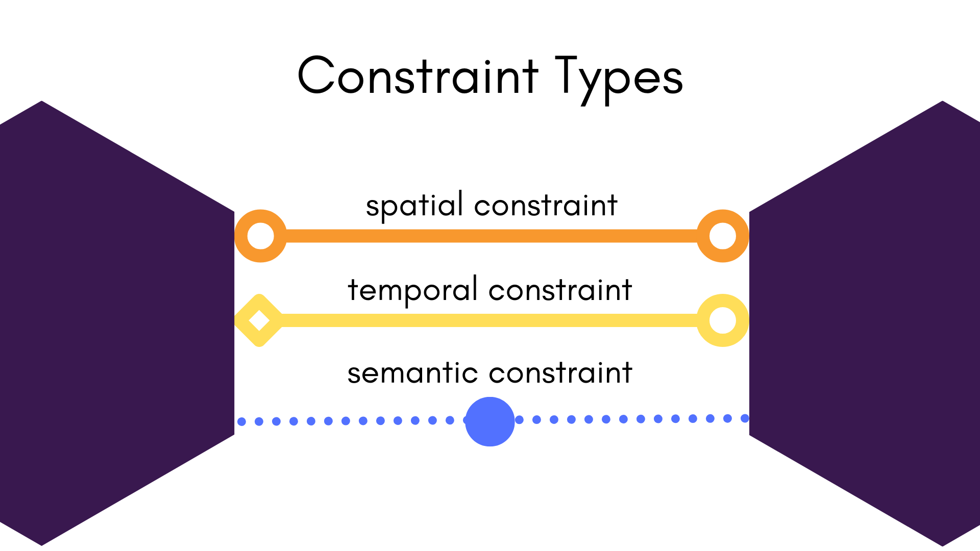
Constraints
A constraint is a spatial, temporal, or semantic relation between any two components. In the context of interpreting plexes as a multigraph of relationships over our system (comprised of different components), constraints are the edge-relationships of the graph.
Conventions
From and To, To and From
Constraints are always across two components. MetriCal will often refer to each of these components in a directional sense using the "from" and "to" specifiers, which reference the UUIDs of the components.
This directional specifier is useful for spatial and temporal constraints, because it allows us to know how the extrinsics from the spatial constraints, or the synchronization data from the temporal constraints can be applied to data to put two observations into the same frame of reference.
Our extrinsics type is essentially a way to describe how to transform points in one coordinate
system into another. Anyone who has ever worked with transforms has experienced confusion in
convention. In order to cut through the ambiguity of extrinsics, every spatial constraint has a
from and to field. Let's dive into how this works.
We can think of an extrinsics transform between components and using the following notation:
If we wanted to move a point from the frame of reference of component to that of , we would use the following math:
...also read as " equals by transforming to from ".
Thus, when constructing a spatial constraint, the reference frame for the extrinsics transform is in the coordinate frame of component , and would move points from the coordinate frame of component .
Similar examples can be made for converting timestamps from e.g. into the same "clock" as using temporal constraints.
Coordinate Bases in MetriCal
It's common to represent a transform in a certain convention, such as FLU (X-Forward, Y-Left, Z-Up) or RDF (X-Right, Y-Down, Z-Forward). One might then wonder what the default coordinate system is for MetriCal. Short answer: it entirely depends on the data you're working with.
In MetriCal, spatial constraints are designed to transform observations (not components!) from the
from frame to the to frame. In the case of a camera-LiDAR extrinsics transform ,
the solved extrinsics will move LiDAR observations (which may be in FLU) to a camera
observations's coordinate frame (which may be in RDF):
This makes it simple to move observations from one component to another for sensor fusion tasks. This is what is meant when MetriCal is said to have no "default" component coordinate system; it operates directly on the provided observations!
However, for those users that really need the extrinsics in a specific coordinate basis, MetriCal provides. There are two relevant global options that can be passed to any mode that produces or displays a calibrated plex (Calibrate, Shape, Pretty Print, and Evaluate). These are:
--topic-to-observation-basis(or-z): Assign a topic a specific coordinate basis for its observations, i.e. the data it produces. For cameras, this is usually RDF.--topic-to-component-basis(or-Z): Assign a topic a specific coordinate basis for its component, i.e. the sensor itself.
If both of these options are set for every component, MetriCal will transform the extrinsics into the proper basis for you! Let's take a look at an example:
metrical calibrate -z ir_cam:RDF -z lidar:FLU -Z *:FLU $DATA $PLEX $OBJ
Here, we're telling MetriCal that the observations from the camera topic are in RDF, while the data from our LiDAR is in FLU. We're also telling MetriCal that we need the output of the entire plex to be in FLU, probably because our system expects that basis natively.
In this case, MetriCal will produce two plexes in the results JSON:
results.plex- The first plex is what is natively produced by the calibration process, with extrinsics in the basis of the observations.results.changed_basis_plex- The second plex is the same as the first, but with all extrinsics transformed into the desired component bases.
Note that this second plex is for your use only; if you use this in Init or Calibrate mode, MetriCal
will probably start a little confused. It needs results.plex for proper operation.
Spatial Constraints
It is common to ask for the spatial relationship or extrinsics between two given components. A Plex incorporates this information in the form of what is called spatial constraints. A spatial constraint can be broken down into:
| Field | Type | Description |
|---|---|---|
| Extrinsics | An extrinsics object | The extrinsics describing the "To" from "From" transformation. |
| Covariance | A matrix of floats | The 6×6 covariance of the extrinsics described by this constraint. |
| From | UUID | The UUID of the component that describes the "From" or base coordinate frame. |
| To | UUID | The UUID of the component that describes the "To" coordinate frame, which we are transforming into. This can be considered the "origin" of the extrinsics matrix |
Spatial Covariance
Spatial covariance is generally presented as a 6×6 matrix relating the variance-covariance of an se3 lie group:
When traversing for spatial constraints within the Plex, the constraint returned will always contain the extrinsic with the minimum overall covariance. This ensures that users will always get the extrinsic that has the smallest covariance (thus, the highest confidence / precision), even if multiple spatial constraints exist between any two components.
Since all spatial constraints in a plex form an undirected (maybe even fully connected) graph, it can be confusing to figure out how to traverse that graph to find the "best" extrinsics between two components. MetriCal itself provides the Shape mode to help with this (with a few helpful options in Pretty Print), but sometimes it's useful to do your own thing.
To help would-be derivers, the
MetriCal Sensor Calibration Utilities
repository contains the spatial_constraint_traversal directory, which demonstrates the right way
to derive optimal extrinsics straight from the Plex JSON via the magic of python.
Temporal Constraints
Time is a tricky thing in perception, but of crucial importance to get right. We've developed our temporal constraint to be flexible enough to describe many of the most common timing scenarios between components.
| Field | Type | Description |
|---|---|---|
| Synchronization | A synchronization object | The strategy to achieve known synchronization between these two components in the Plex. |
| Resolution | float | The resolution to which synchronization should be applied. |
| From | UUID | The UUID of the component that the synchronization strategy must be applied to. |
| To | UUID | The UUID of the component whose clock we synchronize into by applying our synchronization strategy (to the from component). |
The Problem With Clocks
In the world of hardware, measuring time can be a challenge. Two clocks might differ in several different ways; without taking these nuances into account, many higher-level perception tasks can fail.
Let's take the example below: two different clocks, possibly from two different hosts, that might be informing separate components in our plex.
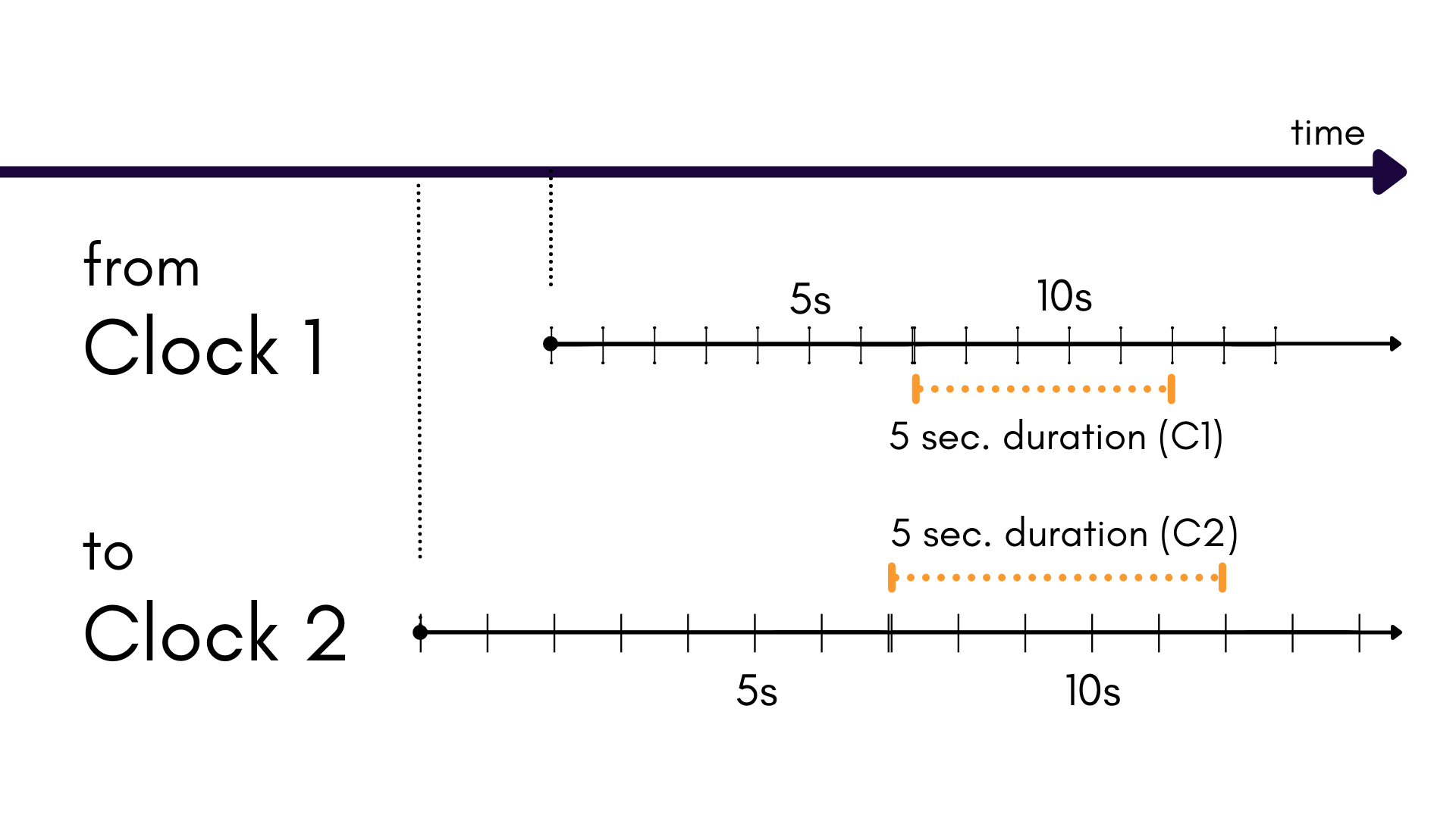
Temporal constraints can balance these different clocks across a plex in order to make sure time confusion never occurs. It achieves this through Synchronization.
Synchronization
Synchronization describes the following relationship between two clocks:
| Field | Type | Description |
|---|---|---|
| offset | Integer | The epoch offset between two clocks, in units of integer nanoseconds. |
| skew | Integer | The scale offset between two clocks. Unitless. |
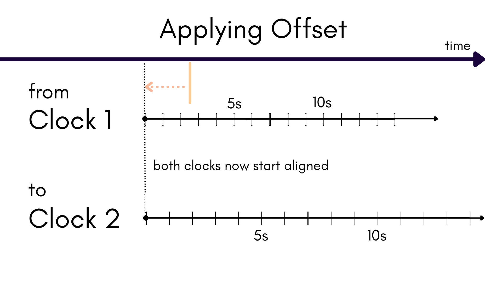
Offset
Unless two components are using the same clock, there's a chance that they are offset in time. This
means that time t in one clock does not align with time t in the other. Fixing this is rather
simple: just shift the time values in the from clock by the offset parameter until their two t
times match.
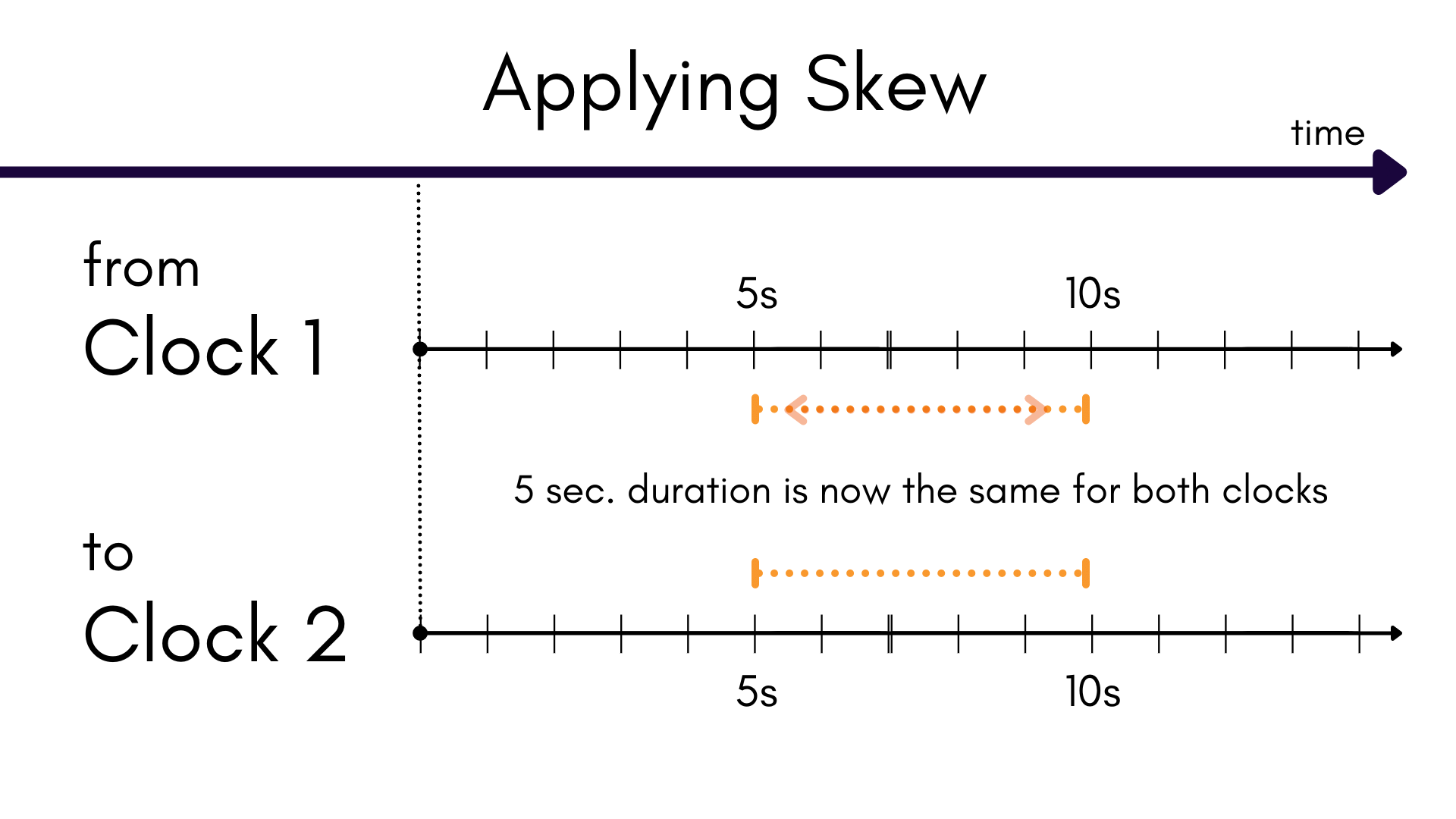
Skew
Skew compensates for the difference in the duration of a time increment between two clocks. In other words, a second in one clock might be a different length than a second in another! These differences can be very subtle, but they will result in some unwanted drift.
Applying skew to a from clock's timestamps will match the duration of a second to that of the
to clock.
Between skew and offset, we have the tools we need to synchronize time between two clocks! Note
that components that use the same host clock will need no synchronization; their skew and offset
remains 0.0.
MetriCal has adopted the terminology from this paper from the University of New Hampshire's InterOperability Laboratory.
Resolution
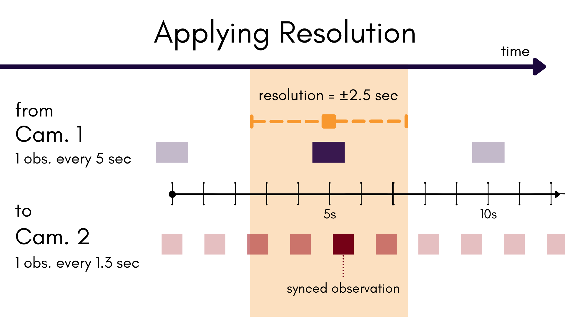
Resolution helps MetriCal identify observations that are meant to be synchronized between two components.
Say we have two camera components. The first is producing one image every 5 seconds; the second produces a new image every 1.3 seconds. We want to pair up observations from the two separate streams that we know are uniquely synced in time as a one-to-one set.
Our resolution tells the Platform how far from an observation we want to search for a synced pair.
In the case of our first camera, we know that one new frame comes every 5 seconds. This means that
there's a span of 2.5 seconds on either side of this image that could hold a matching observation
from our second camera. So, we set resolution to 2.5 * 1e9 (for nanoseconds).
The Platform will then look for any synced observation candidates in camera two and find the observation that matches most closely in time to the image in camera one.
All that being said, resolution is a concept better shown than told:
If one is confident that two observation streams are in-sync, one may set the resolution to be fairly small. However, given the way some components can behave, it's generally not necessary or recommended.
Semantic Constraints
Semantic constraints are a bit different from spatial and temporal constraints. While spatial and temporal constraints exist to model the physical realities of components in a system, semantic constraints exist to model relationships in the system that don't fall within those boundaries.
Semantic constraints are defined by the following fields:
| Field | Type | Description |
|---|---|---|
| Components | An array of component UUIDs | A set of unique UUIDs (corresponding to components that exist within the plex) that are grouped under this semantic. |
| Name | String | The name for these semantics. Usually indicates the purpose or function of the group. |
| UUID | UUID | The unique identifier for the semantic constraint. |
Semantic constraints can label subplexes within a plex, label individual OEM pieces of hardware (e.g. labeling a single Tangram Vision HiFi within a plex), or to group together components that share some common function (e.g. grouping a stereo pair of cameras together).
Some semantic constraints can be used by MetriCal to generate unique kinds of metrics after
calibration. These are identified purely through the semantic constraint's name field. For
example, MetriCal currently understands the following semantic constraint kinds:
"stereo_pair": This denotes that two cameras are part of a stereo pair. This also tells MetriCal to compute stereo rectification metrics after a calibration is complete.