Calibrating Camera-LiDAR

Get the Data

The data used in this tutorial can be found in the MetriCal Sensor Calibration Utilities repository on GitLab.

Objectives

• Record proper data from camera and LiDAR sensors at the same time
• Calibrate the dataset that we have collected
• Analyze the results

---

Next to camera-camera calibration, camera-LiDAR calibration is one of the most common calibration tasks in robotics. Say what you want about their use in vision, but LiDARs bring a ton of valuable spatial information to any perception pipeline. They're even more valuable when used in conjunction with cameras, as the two sensors complement each other's strengths and weaknesses.

We'll be using the following sensor systems in this tutorial:

• One Intel RealSense 435i
• One Livox Mid 70

Recording Data

Using The Circle

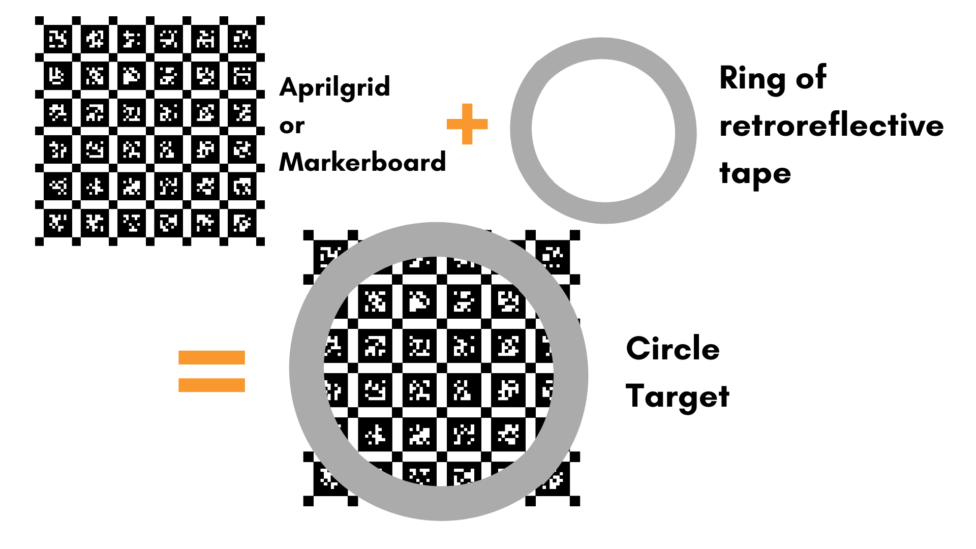
MetriCal uses a special(-to-us) fiducial called a Circular Markerboard, or as we like to call it, the circle. The circle consists of two parts: a markerboard cut into a circle, and retroreflective tape around the edge of the circle. Its design allows MetriCal to bridge the modalities of camera, which is a projection of Euclidean space onto a plane, and LiDAR, which is a representation of Euclidean space.

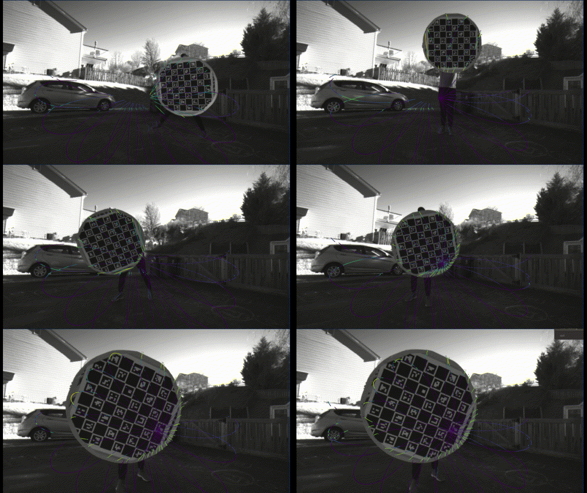
Since we're using a markerboard to associate the camera with a position in space, all of the same data collection considerations for cameras apply:

• Rotate the circle
• Capture several angles
• Capture the circle at different distances

You can read more about proper camera data collection techniques here: Camera Data Capture.

In fact, following those tips will also guarantee that you have good data for LiDAR calibration! LiDAR data collection is more straightforward than camera data collection, only because we're specifically solving for the LiDAR extrinsics alone.

LiDAR Intrinsics

MetriCal doesn't currently calibrate LiDAR intrinsics. if you're interested in calibrating the intrinisics of your LiDAR for better accuracy and precision, get in touch!

Beware the Noise!

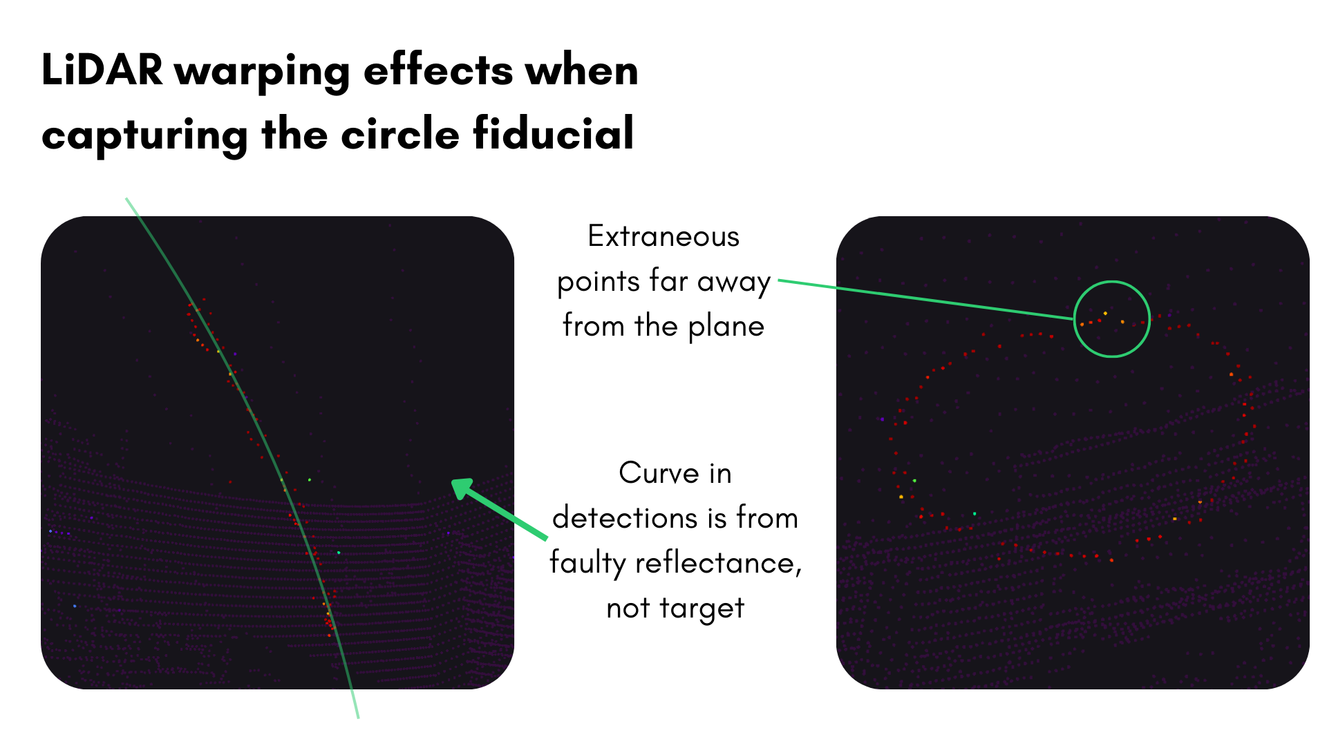
Some LiDAR sensors can have a lot of noise in their data when detecting retroreflective surfaces. This can cause a warping effect in the point cloud data, where the points are spread out in a way that makes it difficult to detect the true surface of the circle. This can be seen most prominently in Ouster rotating LiDARs, like the one used in the image below.

It's not clear if this is an effect of the hardware, firmware, or both, but regardless it can be handled by MetriCal. In order to get the best fit from these readings, it's recommended to set the detect_interior_points flag in the circle detector to false. This way, only the points on the edge of the circle will be used in the calibration.

Pipelining the Data Capture

MetriCal is designed to be a comprehensive calibration tool, and as such, it works best when it's handed all of the data. This includes running the camera calibrations (intrinsics and extrinsics) as well as the LiDAR extrinsics at the same time. This guarantees great accuracy and precision estimates, and generally cuts down on the time spent in calibration.

However, there are circumstances where a great calibration cannot be done in one dataset, e.g. sensors are mounted in places that can't be reached easily by a human operator. In these cases, it's recommended to pipeline the data capture: calibrate each component's intrinsics first, and then use those intrinsics to seed a larger extrinsic calibration.

...But That's For Another Time

Pipeline mode is one way to do this, but there are a few nuances to this procedure that are worth discussing in a separate tutorial.

For now, we'll consider the best case scenario: We were able to capture great data from both cameras and LiDAR that we can use to calibrate everything.

Running MetriCal

As always, running MetriCal takes no time at all:

metrical init -m infra*:no_distortion -m velodyne*:no_offset $DATA $INIT_PLEX
metrical calibrate -v -o $OUTPUT $DATA $INIT_PLEX $OBJ

Here, we've assigned all topics with the infra prefix to use the no_distortion model, since we're assuming that our camera frames are already corrected during streaming. The velodyne prefixed topics are assigned the no_offset model, which is actually the only LiDAR model that is supported in MetriCal at time of writing. This, too, signifies that the LiDAR intrinsics are already known and sufficient. In essence, this Init command is telling MetriCal to only solve for extrinsics.

For Calibrate mode, we've passed in -v to render, and -o to capture the output to the file designated by the $OUTPUT variable. That's about all we need to do here; the vanilla settings for Calibrate mode are fine for us otherwise.

Since we passed the render flag, make sure you have Rerun going in a separate process:

rerun

If your dataset is large (as this one is), you may run into memory issues when running Rerun, especially on resource-limited platforms. By default, Rerun can take up to 75% of total system RAM. To avoid this, you can set a memory limit that's suitable for your machine:

rerun --memory-limit=2GB

Analyzing the Results

Residual Metrics

With camera and LiDAR, MetriCal will output a Circle misalignment RMSE that indicates how well the center of the markerboard (detected in camera space) aligns with the geometric center of the retroreflective circle (in LiDAR space).

If detect_interior_points was set to true, you'll also see Interior point-to-plane RMSE. This metric is a measure of how well the interior points of the circle align with the plane of the circle.

For the dataset in this example, our camera-LiDAR residual metrics are looking pretty good! Here are the derived metrics for our dataset on v9.0:

The root mean square error of our circle misalignment is around 3cm, which is a pretty fair result. The interior point-to-plane error is even better, around 1cm. On paper, it seems like this worked! Let's render it to be sure.

Visualizing the Calibration

During the calibration, two timelines were created in Rerun:

• Detections: This timeline shows the detections of all fiducials in both camera and LiDAR space. Only observations with detections will get rendered; this most likely means you won't see every image in the dataset.
• Corrections: This timeline visualizes the derived calibration as applied to the calibration dataset. It also visualizes the object space and all of its spatial constraints.

Together, these two timelines give a comprehensive view of the calibration process. You can find and toggle these timelines in the bottom left corner of the Rerun interface.

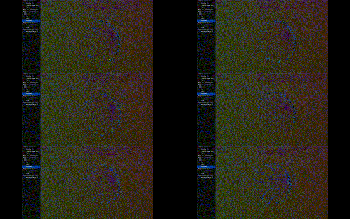
The detections pipeline is pretty straightforward. However, it's worth mentioning that you can focus in on the LiDAR detections by double-clicking on detections for an even closer look at the circle:

The corrections pipeline is where the magic happens. Double-clicking on a camera in the corrections space in the left sidebar will show the aligned camera-LiDAR view. Sure enough, this seems to be a pretty good calibration! The LIVOX's sweeping patterns are clearly visible in the camera space, and the camera's view is looking rectilinear.

Of course, "pretty good" is subjective. The accuracy and precision MetriCal derived from your data may not work for your system! In that case, recapturing data at a slower pace, or with a modified fiducial with more/less retroreflectivity may be necessary.