LiDAR ↔ LiDAR Calibration

LiDAR Circle Target

All of MetriCal's LiDAR calibrations require a circle target to be used in the object space.

Practical Example

We've captured an example of a good LiDAR ↔ LiDAR calibration dataset that you can use to test out MetriCal. If it's your first time performing a LiDAR calibration using MetriCal, it might be worth running through this dataset once just so that you can get a sense of what good data capture looks like.

Running the Example Dataset

First, download the dataset here and unzip it somewhere on your computer. Then, copy the following bash script into the dataset directory:

warning

This script assumes that you have either installed the apt version of MetriCal, or that you are using the docker version with an alias set to metrical. For more information, please review the MetriCal installation instructions.

#!/bin/bash -i
DATA=./lidar_lidar2.mcap
INIT_PLEX=init_plex.json
OBJ=object.json
OUTPUT=results.json
REPORT=results.html

# Front cameras
metrical init \
    -y \
    -m *livox*:lidar \
    -m *points*:lidar \
    $DATA $INIT_PLEX
metrical calibrate \
    --render \
    --report-path $REPORT \
    -o $OUTPUT $DATA $INIT_PLEX $OBJ

The metrical init command uses the -m flag to describe the system being calibrated. It indicates that any topics containing the words livox or points are our lidar topics. We can use the * glob character to capture multiple topics, or to just prevent extra typing when telling MetriCal which topics to use. The configuration generated by metrical init is saved to a file named plex.json, which will be used during the calibration step to configure the system. You can learn more about plexes here.

Finally, note the --render flag being passed to metrical calibrate. This flag will allow us to watch the detection phase of the calibration as it happens in realtime. This can have a large impact on performance, but is invaluable for debugging data quality issues. Rendering has been enabled here so that you can watch the dataset as it's being processed.

warning

MetriCal depends on Rerun for all of its rendering. As such, you'll need a specific version of Rerun installed on your machine to use the --render flag. Please ensure that you've followed the visualization configuration instructions before running this script.

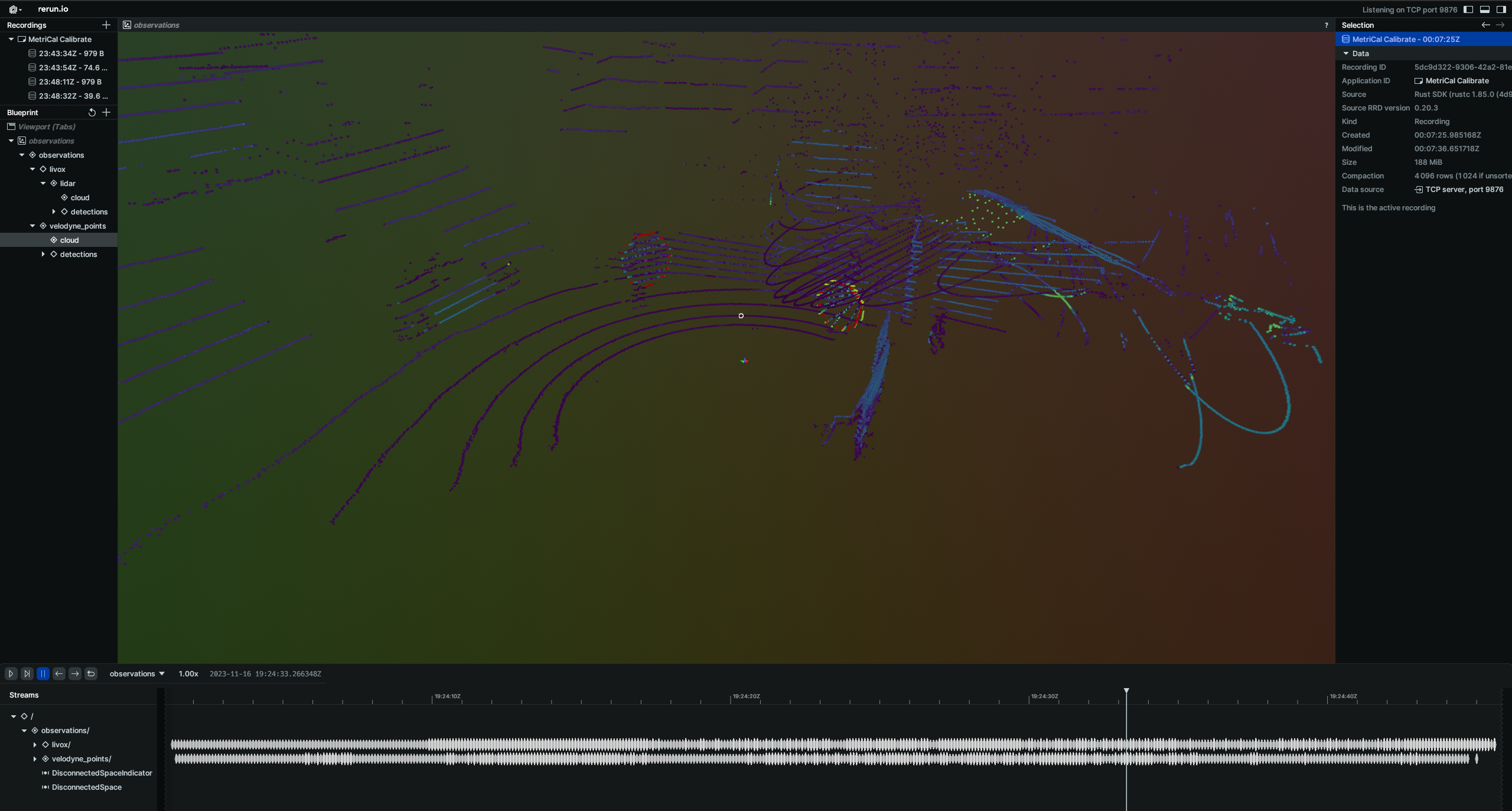
You should now be ready to run the script. When you start it, it will display a visualization window like the following with two LiDAR point clouds in the same coordinate frame (but not registered to one another yet). Note that the LiDAR circle detections will show up as red points in the point cloud.

While the calibration is running, take specific note of the target motion patterns, presence of still periods, and breadth of coverage. When it comes time to design a motion sequence for your own systems, try to apply any learnings you take from watching this capture.

When the script finishes, you'll be left with three artifacts:

• plex.json - as described in the prior section.
• report.html - a human-readable summary of the calibration run. Everything in the report is also logged to your console in realtime during the calibration. You can learn more about interpreting the report here.
• results.json - a file containing the final calibration and various other metrics. You can learn more about results json files here and about manimulating your results using shape commands here.

And that's it! Hopefully this trial run will have given you a better understanding of how to capture your own LiDAR ↔ LiDAR calibration.

Data Capture Guidelines

Many of the tips for LiDAR ↔ LiDAR data capture are similar to Camera ↔ LiDAR capture. Below we've outlined best practices for capturing a dataset that will consistently produce a high-quality calibration between two LiDAR components.

Best Practices

DO	DON'T
✅ Vary distance from sensors to target to capture a wider range of readings.	❌ Stand at a single distance from the sensors.
✅ Ensure good point density on the target for all LiDAR sensors.	❌ Only capture poses where the target does not have sufficient point density.
✅ Rotate the target on its planar axis to capture poses at different orientations.	❌ Keep the board in a single orientation for every pose.
✅ Maximize convergence angles by angling the target up/down and left/right during poses.	❌ Keep the target in a single orientation, minimizing convergence angles.
✅ Pause in between poses (1-2 seconds) to eliminate motion artifacts.	❌ Move the target constantly or rapidly during data capture.
✅ Achieve convergence angles of 35° or more on each axis when possible.

Maximize Variation Across All 6 Degrees Of Freedom

When capturing the circular target with multiple LiDAR components, ensure that the target can be seen from a variety of poses by varying:

• Roll, pitch, and yaw rotations of the target relative to the LiDAR sensors
• X, Y, and Z translations between poses

MetriCal performs LiDAR-based calibrations best when the target can be seen from a range of different depths. Try moving forward and away from the target in addition to moving laterally relative to the sensors.

The field of view of a LiDAR component is often much greater than a camera, so be sure to capture data that fills this larger field of view.

Troubleshooting

If you encounter errors during calibration, please refer to our Errors documentation.

Common issues with LiDAR ↔ LiDAR calibration include:

• No features detected (cal-calibrate-001)
• Too many component observations filtered (cal-calibrate-006)
• Compatible component type has no detections (cal-calibrate-008)

Remember that when working with multiple LiDAR sensors, it's important to ensure all sensors can clearly see the calibration target throughout the data capture process.