Console Log
When calibrating with MetriCal, the metrical calibrate command writes a ton of helpful logs to
stderr (depending on your log level). These are useful for debugging and
understanding the calibration process.
If you'd like to preserve these in an HTML format for easy debugging, pass the
--report-path option to any metrical run.
Pre-Calibration Metrics
MetriCal will output several tables before running the full calibration. Many of these tables can
help determine how useful a dataset will be for calibration. When the --interactive flag is used
during a metrical calibrate run, the process will pause completely and wait for user feedback
before running the calibration itself.
With Detections
This table shows the
- Total observation count from all components
- The total observation count after motion filtering (if set), out of the total observation count
- The total observation count with features in view, out of the filtered set
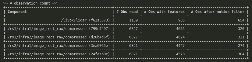
This can be a useful heuristic to check if the motion filter is filtering too aggressively, or if the object space isn't being viewed by any components.
Binned Coverage Count
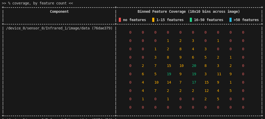
This chart demonstrates how many features were detected in each "bin" in a 10×10 grid representing the image extent. As is shown in this snapshot, the colors of the feature counts shift from red (bad feature coverage) to blue (excellent feature coverage). In general when capturing data, these feature coverage charts should ideally be green to blue in every bin.
It may not always be possible to achieve the "best" possible coverage. In such cases, it is recommended that you fill the image extent as much as is practical.
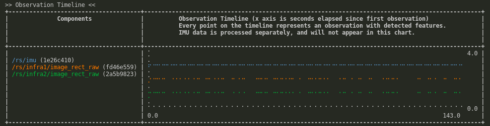
Observation Timeline
| Axis | Description |
|---|---|
| X | The timestamp of the observations, starting from 0 |
| Y | Each component |
The observation timeline table just what it says on the tin: the timestamps of all observations from each component mapped onto the same chart. MetriCal sets the earliest timestamp as 0; timestamps increase monotonically.
This table is useful for determining if observations are synced together properly. If you expect all of your observations to align nicely, but they aren't aligned at all, it's a sign that
- The timestamps are not being written or read correctly
- The temporal constraints in your Plex are incorrect
Either way, this table is a good place to start debugging.
Post-Calibration Metrics
Cameras
Camera Summary Stats
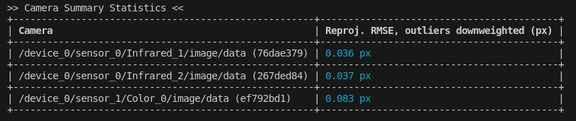
The Camera Summary Statistics show the Root Mean Square Error (RMSE) of the Image Reprojection for each camera in the calibration. For a component that has been appropriately modeled (i.e. there are no un-modeled systematic error sources present), this represents the mean quantity of error from observations taken by a single component.
Units for RMSE are specific to the component in question, and should not necessarily be compared directly. For example, camera components will be making observations in units of pixels in image space, which means our RMSE is in units of pixels as well.
If two cameras have pixels of different sizes, then it is important to first convert these RMSEs
to some metric size so as to compare them equally. This is what pixel_pitch in the
Plex API is for: cameras can be compared more equally with that
in mind, as the pixel size between two cameras is not always equal!
Camera Intrinsics
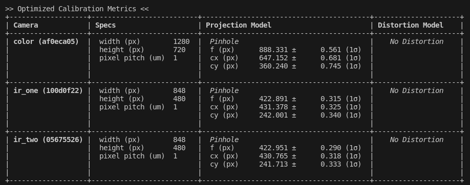
This table is exactly what it claims to be: a summary of the intrinsics of each camera in the dataset. Different models will have different interpretations; see the Camera Models page for more.
Binned Reprojection Errors
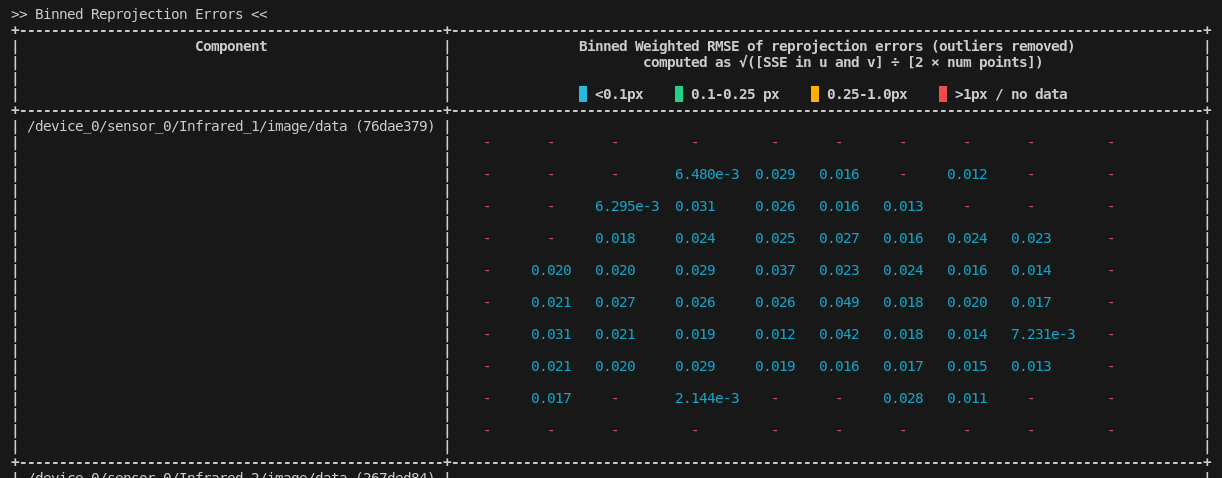
Similar to the binned coverage charts in the pre-calibration, the binned reprojection errors display a similar representation except the collective reprojection RMSE (root-mean-square-error) is printed instead of the total feature count.
Like the coverage charts, this is color-coded from red (bad, large reprojection errors) to blue (excellent reprojection errors). In most calibrations, the aim will probably be to get this number as low as possible.
Our color coding is merely a guideline. You should set your own internal tolerances for this sort of metric.
Stereo Pair Rectification Error
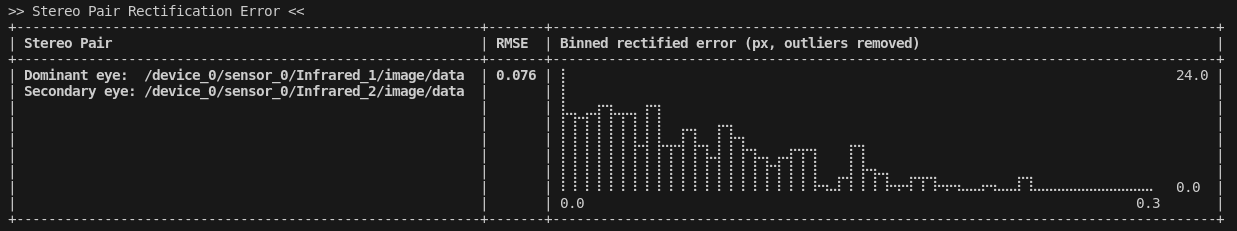
| Axis | Description |
|---|---|
| X | The reprojection error in pixels |
| Y | The number of observations with that reprojection error |
Since stereo rectification is such a common part of camera calibration, MetriCal will label any pairs of cameras that fit the following criteria as a stereo pair:
- The cameras are facing the same way, up to a 5° tolerance
- The camera translation in X (right-left w.r.t. camera orientation) or Y (up-down) is at least 10x the length of the translation in any other axis
- The cameras are the same resolution
From there, MetriCal will run rectification process on every synced image pair in the dataset and calculate the reprojection error in the Y-axis.
Lidar
LiDAR Summary Stats
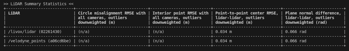
The LiDAR Summary Statistics show the Root Mean Square Error (RMSE) of four different types of residual metrics:
- Circle Misalignment, if a camera-lidar pair is co-visible with a circular markerboard.
- Interior Points to Plane Error, if a camera-lidar pair is co-visible with a circular markerboard.
- Paired 3D Point Error, if a lidar-lidar pair is co-visible with a circular markerboard.
- Paired Plane Normal Error, if co-visible LiDAR are present
For a component that has been appropriately modeled (i.e. there are no un-modeled systematic error sources present), this represents the mean quantity of error from observations taken by a single component.
In the snapshot above, notice that the two LiDAR have the same RMSE relative to one another. This makes intuitive sense: LiDAR A will have a certain relative error to LiDAR B, but LiDAR B will have that same relative error when compared to LiDAR A. Make sure to take this into account when comparing LiDAR RMSE more generally.
IMU
Optimized IMU Metrics
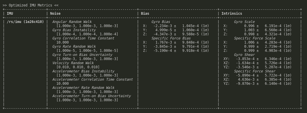
This table presents all IMU metrics derived for every IMU component in a calibration run. The most interesting column for most users is the Intrinsics: scale, shear, rotation, and g sensitivity.
Extrinsics
Minimum Spanning Tree
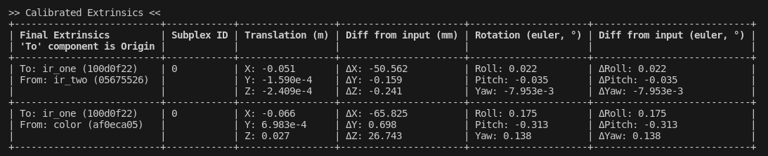
This table represents the Minimum Spanning Tree of all spatial constraints in the Plex. Note that this table doesn't print all spatial constraints in the plex; it just takes the "best" constraints possible that would still preserve the structure.
Rotations are printed as Euler angles, using Extrinsic XYZ convention.
Component Extrinsics Errors
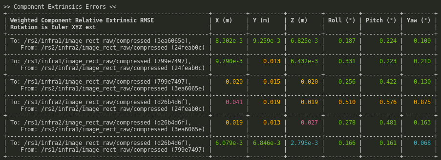
This is a complete summary of all component extrinsics errors (as RMSE) between each pair of components, as described by the Composed Relative Extrinsics metrics. This table is probably one of the most useful when evaluating the quality of a plex's extrinsics calibration. Note that the extrinsics errors are weighted, which means outliers are taken into account.
Rotations are printed as Euler angles, using Extrinsic XYZ convention.
IMU Preintegration Errors
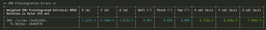
This is a complete summary of all IMU Preintegration errors from the system. Notice that IMU preintegration error is with respect to an object space, not a component. The inertial frame of a system is tied to a landmark in space, so it makes sense that an IMU's error would be tied to a fiducial.
Rotations are printed as Euler angles, using Extrinsic XYZ convention.
Optimization Summary Stats

These statistics are a (loose) picture of the overall quality of the calibration data. A bad posterior variance, or a very high object space error, may indicate that something was wrong with the data or the fiducial setup. Ultimately, however, these are just heuristics and should be taken as just part of the picture.
Optimized Object Space RMSE
This is a measurement of how the dimensions of the fiducials as described in the object space differed from their solved positions in the optimization. Since cameras produce the only observations that allow MetriCal to calculate this deformation, the RMSE is in units of pixels.
Posterior Variance
Also known as "a-posteriori variance factor" or "normalized cost," the posterior variance is a relative measure of the gain/loss of information from the calibration.
Uncertainty is necessarily a measure of precision, not accuracy. Prior and posterior variance tell us about the data that we observed and its relation to the model we chose for our calibration, but doesn't say anything about the accuracy of the model itself.
Posterior variance doesn't make sense without discussing prior variance, or the "a-priori variance factor". Prior variance in MetriCal is a global scale on the uncertainty of our input data. This could be considered a relative measure of confidence in a given "geometric network" of data input into our calibration.
MetriCal always starts with a prior variance of 1.0 in the adjustment — in other words, no calibration is considered special with regards to its input uncertainty. MetriCal will just use default uncertainties for any given observed quantity and scale the whole "network" with 1.0.
This means that the posterior variance is only useful when compared to the prior, or 1.0. Posterior variance can be computed in any least-squares adjustment by using the following formula:
where is the residuals vector, is the covariance matrix of the observations in the calibration, and D.o.F. refers to the total degrees of freedom in the entire adjustment. The upper part of the above fraction is the cost function of a least-squares process (the weighted square sum of residuals), which is why this is sometimes referred to as "normalized cost."
Posterior vs Prior Variance
The trick here is in interpreting this value relative to our prior variance of 1.0. There are three possible scenarios that can occur:
- Posterior variance is approximately 1.0 ( = 1.0)
- Posterior variance is less than the prior variance ( < 1.0)
- Posterior variance is greater than the prior variance ( > 1.0)
The first scenario is the simplest, but also the least interesting. If the posterior variance matches the prior variance well, then our uncertainty has been correctly quantified, and that the final variances of our estimated parameters match expectations.
In the second, the residual error across the data set is now smaller than what was expected. This could mean the problem was pessimistic in its initial estimate of uncertainty in the problem definition. Taking a more Bayesian approach, it can be interpreted as having more information or certainty in the results of the calibration using this data set than it had going in.
The posterior variance is now larger than what was expected at the outset. This implies the opposite of Posterior < Prior: the problem was optimistic in its initial estimate of uncertainty. In other words, we now have more uncertainty (less certainty) in the results using this data set than we thought we ought to have, after considering the data.
What's Best?
From the latter two scenarios, it might be tempting to say that posterior variance should always be less than or equal to 1.0. After all, it should be better to remain pessimistic or realistic with regards to our uncertainty than it is to be optimistic and have more error, right?
Unfortunately, this is a very broad brush with which to explain our posterior variance. This kind of naive explanation may lead to some biased inferences; in particular, there's a good number of reasons why posterior variance might be smaller than prior variance:
- We set our prior variances to be very large, and that was unrealistic.
- The data set contained much more data than was necessary to estimate the parameters to the appropriate level of significance. This relates to the observability of our parameters as well as the number of parameters we are observing.
Conversely, there's a number of good reasons for why posterior variance may be larger than prior variance:
- The prior variance was set to be very small, and that was unrealistic. This can occur if the data set is good, but observations from the data are qualitatively bad for some reason (e.g. a blurry lens that was installed incorrectly). The model and data would not agree, so residual error increases.
- The data set did not contain enough degrees of freedom (D.o.F) to be able to minimize residuals to the level of desired significance. This can occur when individual frames in a camera do not detect enough points to account for the number of parameters we have to estimate for that pose / frame / intrinsics model / etc.
- The data actually disagrees with prior estimates of our parameters. This can occur if parameters are "fixed" to incorrect values, and the data demonstrates this through larger residual error. This can also occur when there are large projective compensations in our model, and our data set does not contain frames or observations that would help discriminate correlations across parameters.
It is easy to misattribute any one of these causes to a problem in the calibration; for instance, if the model and correspondent covariances in the plex are acceptable and the other calibration outputs don't show any signs that the calibration is invalid in some way, then posterior variance likely will not reveal any new insight into the calibration.
Generally speaking, posterior variance needs to differ by quite a large margin before it is worth worrying about, and you'll likely see other problems in the calibration process that will lead to more fruitful investigations if something is "wrong" or can be improved upon.
As a rule of thumb, if posterior variance isn't less than or greater than 3.0 (a factor of 3 between posterior and prior variance), then you shouldn't worry about it.