Image Reprojection
Overview
Reprojection error is the error in the position of a feature in an image, as compared to the position of its corresponding feature in object space. More simply put, it tells you how well the camera model generalizes in the real world.
Reprojection is often seen as the only error metric to measure precision within an adjustment. Reprojection errors can tell us a lot about the calibration process and provide insight into what image effects were (or were not) properly calibrated for.
Definition
Image reprojection metrics contain the following fields:
Field | Type | Description |
|---|---|---|
metadata | A common image metadata object | The metadata associated with the image that this reprojection data was constructed from. |
object_space_id | UUID | The UUID of the object space that was observed by the image this reprojection data corresponds to. |
ids | An array of integers | The identifiers of the object space features detected in this image. |
us | An array of floats | The u-coordinates for each object space feature detected in this image. |
vs | An array of floats | The v-coordinates for each object space feature detected in this image. |
rs | An array of floats | The radial polar coordinates for each object space feature detected in this image. |
ts | An array of floats | The tangential polar coordinates for each object space feature detected in this image. |
dus | An array of floats | The error in u-coordinates for each object space feature detected in this image. |
dvs | An array of floats | The error in v-coordinates for each object space feature detected in this image. |
drs | An array of floats | The error in radial polar coordinates for each object space feature detected in this image. |
dts | An array of floats | The error in tangential polar coordinates for each object space feature detected in this image. |
world_extrinsic | An extrinsics object | The pose of the camera (camera from object space) for this image. |
object_xs | An array of floats | The object space (3D) X-coordinates for each object space feature detected in this image. |
object_ys | An array of floats | The object space (3D) Y-coordinates for each object space feature detected in this image. |
object_zs | An array of floats | The object space (3D) Z-coordinates for each object space feature detected in this image. |
rmse | Float | Root mean square error of the image residuals, in pixels. |
Camera Coordinate Frames
MetriCal uses two different conventions for image space points. Both can and should be used when analyzing camera calibration statistics.
CV (Computer Vision) Coordinate Frame
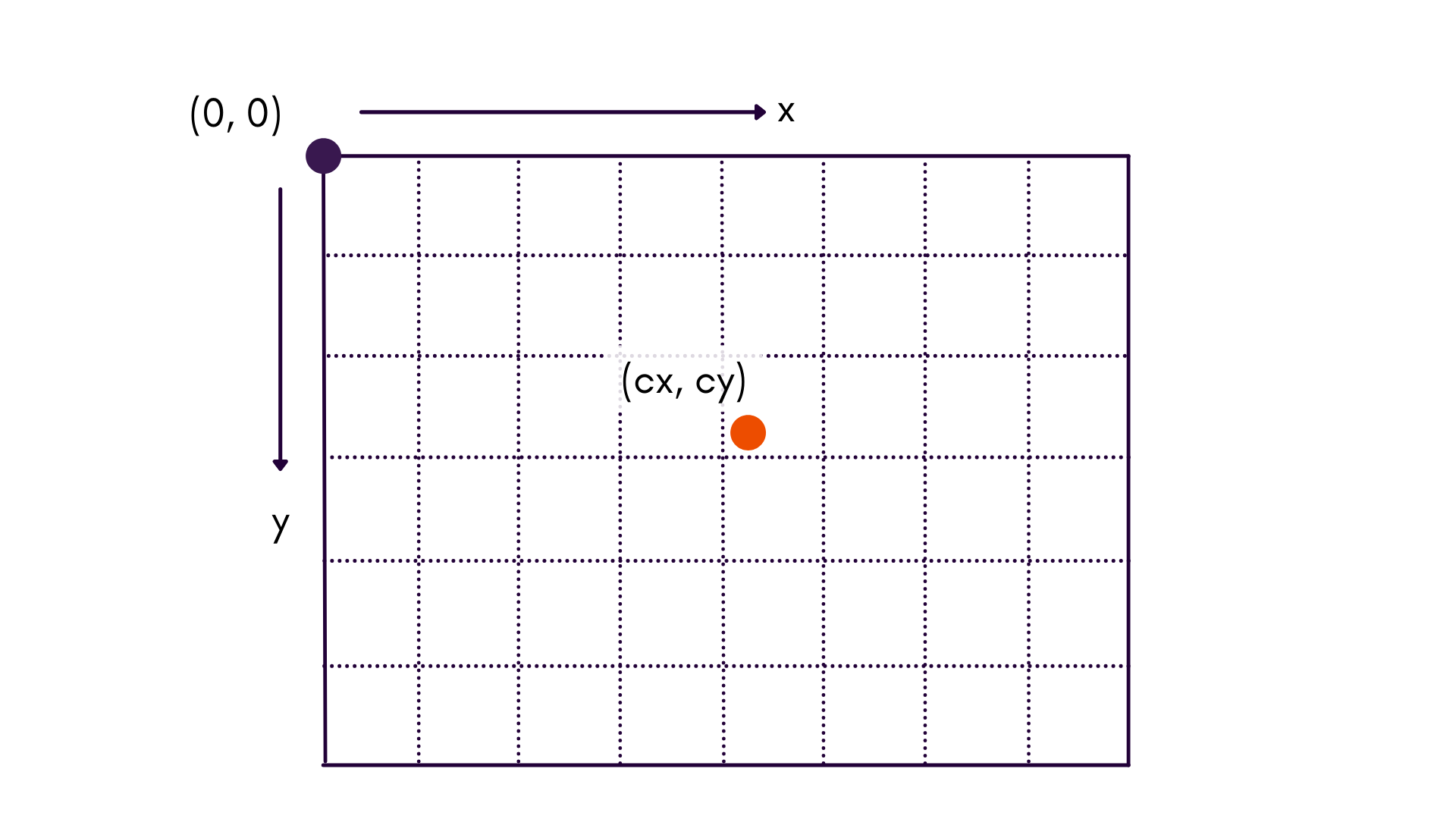
This is the standard coordinate system used in computer vision. The origin of the coordinate system is , and is located in the upper left corner of the image.
When working in this coordinate frame, we use lower-case and to denote that these coordinates are in the image, whereas upper-case , , and are used to denote coordinates of a point in object space.
This coordinate frame is useful when examining feature space, or building histograms across an image.
UV Coordinate Frame
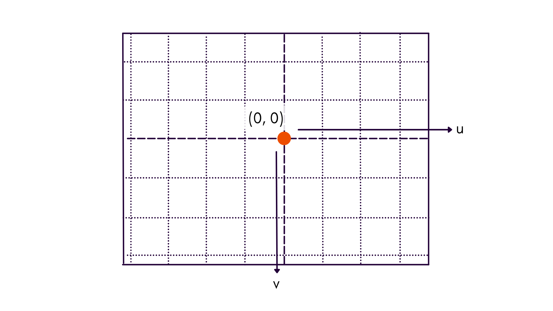
This coordinate frame maintains axes conventions, but instead places the origin at the principal point of the image, labeled as . Notice that the coordinate dimensions are referred to as lower-case and , to denote that axes are in image space and relative to the principal point.
Most charts that deal with reprojection error convey more information when plotted in UV coordinates than CV coordinates. For instance, radial distortion increases proportional to radial distance from the principal point — not the top-left corner of the image.
Cartesian vs. Polar
In addition to understanding the different origins of the two coordinate frames, polar coordinates are sometimes used in order to be able to visualize reprojections as a function of radial or tangential differences.
When using polar coordinates, points are likewise centered about the principal point. Thus, we go from our previous frame to .
| Cartesian | Polar |
|---|---|
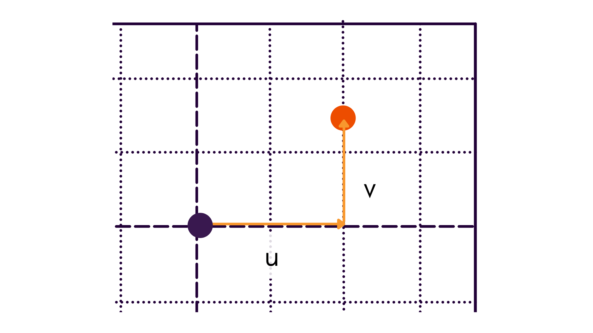 | 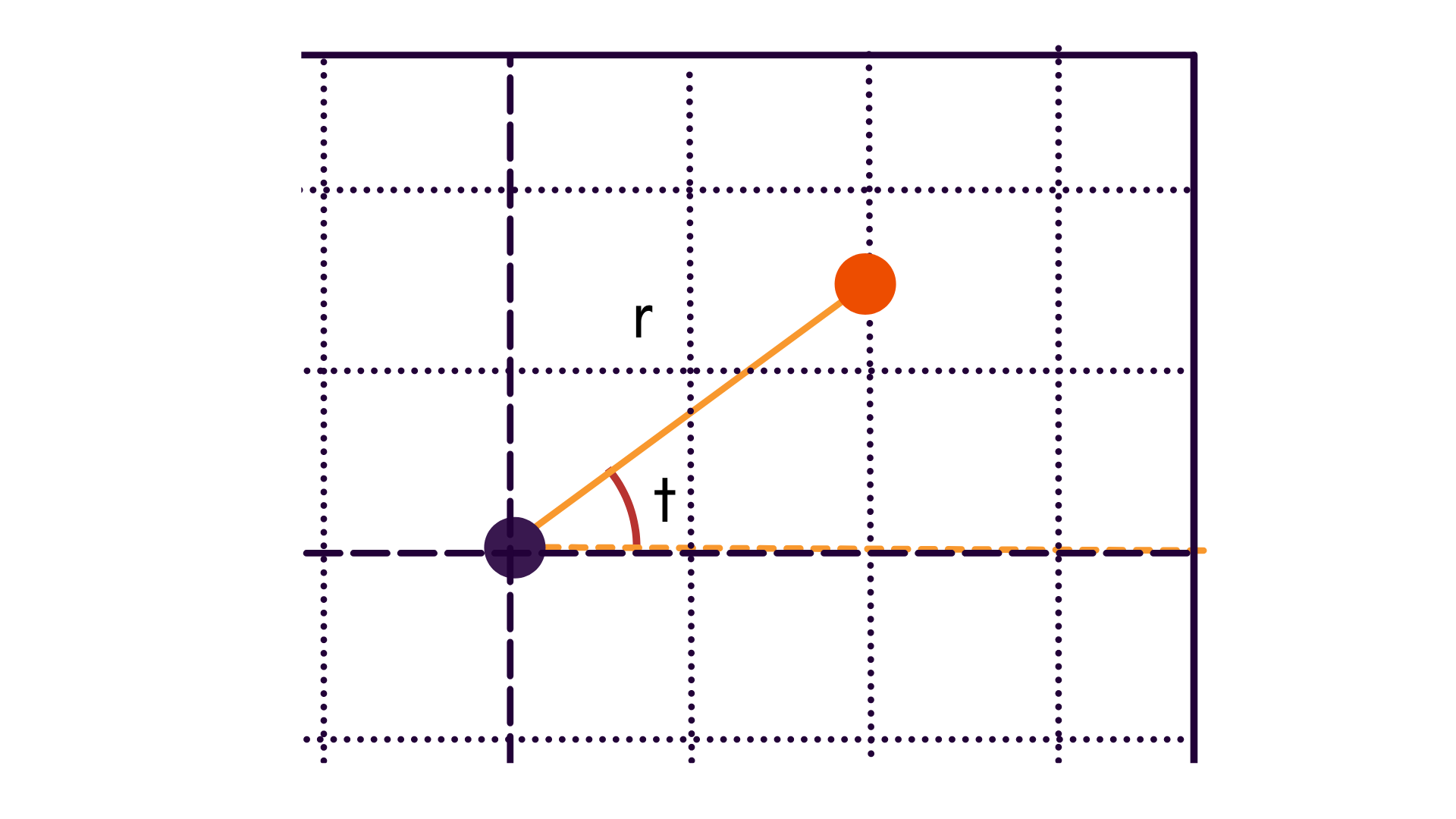 |
Analysis
Below are some useful reprojection metrics and trends that can be derived from the numbers found in
results.json.
Feature Coverage Analysis
Data Based In: Either CV or UV Coordinate Frame
All image space observations made from a single camera component over the entire calibration process are plotted. This gives us a sense of data coverage over the domain of the image. For a camera calibration process, this chart should ideally have an isometric distribution of points within the image without any large empty spaces. This even spread prevents a camera model from overfitting on any one area.
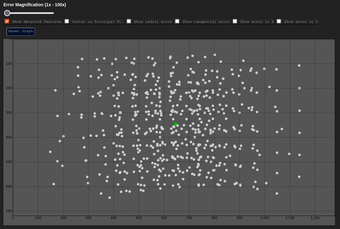
In the above example, there are some empty spaces near the periphery of the image. This can happen due to image vignetting (during the capture process), or just merely because one did not move the target to have coverage in that part of the scene during data capture.
Radial Error - δr vs. r
Data Based In: UV Coordinate Frame
The vs. graph is a graph that plots radial reprojection error as a function of radial distance from the principal point. This graph is an excellent way to characterize distortion error, particularly radial distortions.
| Expected | Poor Result |
|---|---|
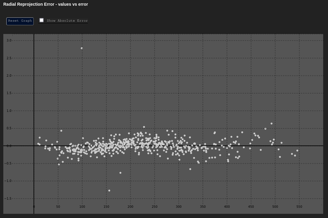 |  |
Consider the graph above: This distribution represents a fully calibrated system that has modeled distortion using the Brown-Conrady model. The error is fairly evenly distributed and low, even as one moves away from the principal point of the image.
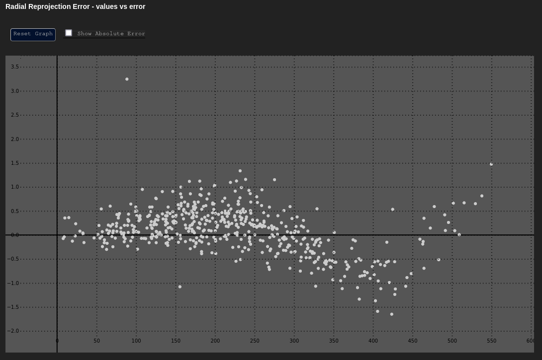
However, were MetriCal configured to not to calibrate for a distortion model (e.g. a plex was
generated with metrical init such that it used the no_distortion model), the output would look
very different (see the right figure above). Radial error fluctuates in a sinusoidal pattern now,
getting worse as we move away from the principal point. Clearly, this camera needs a distortion
model of some kind in future calibrations.
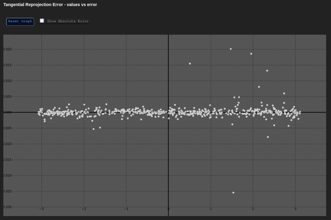
Tangential Error - δt vs. t
Data Based In: UV Coordinate Frame
Like the vs. graph, vs. plots the tangential reprojection error as a function of the tangential (angular) component of the data about the principal point.
This can be a useful plot to determine if any unmodeled tangential (de-centering) distortion exists. The chart below shows an adjustment with tangential distortion correctly calibrated and accounted for. The "Poor Result" shows the same adjustment without tangential distortion modeling applied.
| Expected | Poor Result |
|---|---|
 | 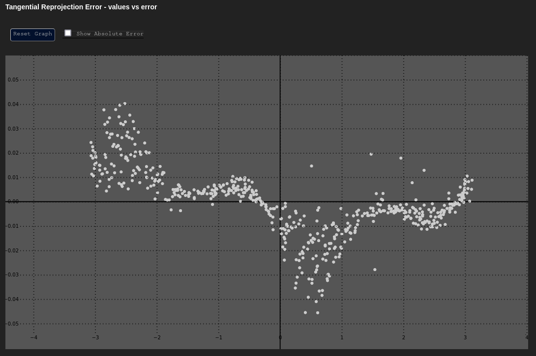 |
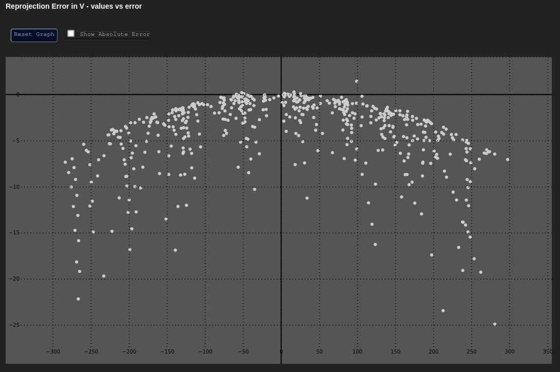
Error in u and v
Data Based In: UV Coordinate Frame
These plot the error in our Cartesian axes ( or ) as a function of the distance along that axis ( or ).
Both of these graphs should have their y-axes centered around zero, and should mostly look uniform in nature. The errors at the extreme edges may be larger or more sparse; however, the errors should not have any noticeable trend.
| Expected δu vs. u | Expected δv vs. v |
|---|---|
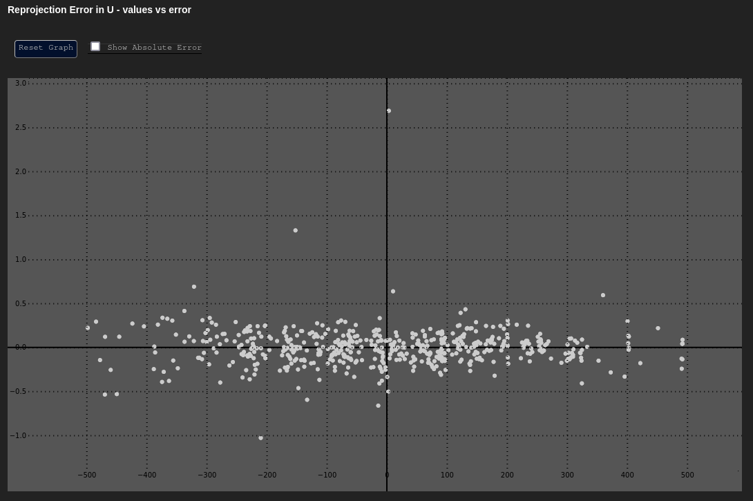 | 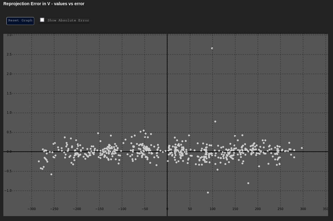 |
Unmodeled Intrinsics Indicators
There are certain trends and patterns to look out for in the plots above. Many of these can reveal unmodeled intrinsics within a system, like a distortion that wasn't taken into account in this calibration process. A few of these patterns are outlined below.
Unmodeled Tangential Distortion
It was obvious that something was amiss when looking at the Poor Result plot for the vs. graph, above. However, depending on the magnitude of error, we may suspect that any effects we see in such a graph are noise. If we then look at the vs. and vs. graphs, we might see the following trends as well:
| Unmodeled Tangential - δu vs. u | Unmodeled Tangential - δv vs. v |
|---|---|
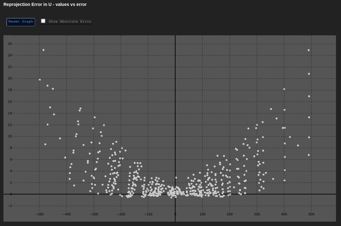 |  |
Comparative Analysis
Beyond the above analyses, the charts provided are incredibly useful when comparing calibrations for the same component over time. Comparing these charts temporally is useful when designing a calibration process, and likewise can be useful in deciding between different models (e.g. Brown-Conrady vs. Kannala-Brandt distortion, etc.).
Comparing these charts across components can be helpful if the components are similar (e.g. similar cameras from the same manufacturer). There are some caveats; for example, one cannot compare these charts across two cameras if they have different pixel pitches. Pixel errors from a camera that has 10µm pixels cannot be directly compared to pixel errors from a camera that has 5µm pixels, as the former is 2 times larger than the latter. One might understandably see that the former component has reprojection errors 2 times smaller than the latter, but this would be a false distinction — that difference is due to the difference in size between the pixels of both cameras and not due to some quality of the calibration.
Pose Data
The world_extrinsic from the image reprojection data represents the pose (camera from object
space) of the camera when a given image was taken. Knowing which image is which by uniquely
identifying it by its component UUID and timestamp (present in the metadata), these poses can be
plotted or used to determine the position of the camera when a given image was taken.
This is one way to perform a hand-eye calibration with MetriCal, by extracting the world pose of each image given a timestamp or sequence number.
Object XYZs
In addition to image reprojections, the final "unprojected" 3D coordinates of the object space features are also included in image reprojection metrics. This can be used in conjunction with other modality information to determine how an individual image contributed to errors in the final optimized object space.
While MetriCal does not have any means to single out and filter an individual image, this can help during the development of a calibration process to ascertain if certain poses or geometries negatively contribute towards the calibration.